It is a common task to find datasets which have different types of variables, and they could be numeric, time data, or even categorical. The inspectdf package offers a set of functions to analyze the behavior of this kind of data.
First of all, we have to install the package.
library(devtools)
install_github("alastairrushworth/inspectdf")
When we installed the package, it is necessary to load it. We do the same with dplyr package, especially for use the pipe %>%.
library(inspectdf)
library(dplyr)
For this example, the dataset starwars will be used. This dataset is in dplyr package and which has data from various characters in this cinematographic universe.
starwars %>%
    head()
## # A tibble: 6 x 14
## name height mass hair_color skin_color eye_color birth_year sex gender
## <chr> <int> <dbl> <chr> <chr> <chr> <dbl> <chr> <chr>
## 1 Luke~ 172 77 blond fair blue 19 male mascu~
## 2 C-3PO 167 75 <NA> gold yellow 112 none mascu~
## 3 R2-D2 96 32 <NA> white, bl~ red 33 none mascu~
## 4 Dart~ 202 136 none white yellow 41.9 male mascu~
## 5 Leia~ 150 49 brown light brown 19 fema~ femin~
## 6 Owen~ 178 120 brown, gr~ light blue 52 male mascu~
## # ... with 5 more variables: homeworld <chr>, species <chr>, films <list>,
## # vehicles <list>, starships <list>Tabular exploratory data analysis
The inspectdf package allows you to calculate some descriptive statistics quickly for any variable using theinspect_types()function.
starwars %>%
    inspect_types()
## # A tibble: 4 x 4
## type cnt pcnt col_name
## <chr> <int> <dbl> <named list>
## 1 character 8 57.1 <chr [8]>
## 2 list 3 21.4 <chr [3]>
## 3 numeric 2 14.3 <chr [2]>
## 4 integer 1 7.14 <chr [1]>The previous result shows that there are seven variables of type character, which represents 53.84% of the dataset. Also, there are two numerical variables, which represent 15.38%. The above is useful for a first look, but it is interesting to go a little further and describe all the variables in more detail. For this, the inspect_cat () function could be useful.
starwars %>%
    inspect_cat()
## # A tibble: 8 x 5
## col_name cnt common common_pcnt levels
## <chr> <int> <chr> <dbl> <named list>
## 1 eye_color 15 brown 24.1 <tibble [15 x 3]>
## 2 gender 3 masculine 75.9 <tibble [3 x 3]>
## 3 hair_color 13 none 42.5 <tibble [13 x 3]>
## 4 homeworld 49 Naboo 12.6 <tibble [49 x 3]>
## 5 name 87 Ackbar 1.15 <tibble [87 x 3]>
## 6 sex 5 male 69.0 <tibble [5 x 3]>
## 7 skin_color 31 fair 19.5 <tibble [31 x 3]>
## 8 species 38 Human 40.2 <tibble [38 x 3]>The inspect_cat () function shows in the first column the name of the variable, in the second one the number of unique values it contains, that is, the variable * eye_color * has 15 different levels, or what is the same, there are 15 colors and different eyes in the database. The third column shows the most common value that appears in the variable; for example, the most common species that appear in the dataset are humans. The fourth column indicates the percentage that represents the most common level; for example, the brown eyes represent 24.13% of all the colors present in the data. So what does the fifth column represent? Well, it is a list with the proportions of each level of the variable. Consider the * df * object from the previous result.
df <- starwars %>%
    inspect_cat()
df$levels$eye_color
## # A tibble: 15 x 3
## value prop cnt
## <chr> <dbl> <int>
## 1 brown 0.241 21
## 2 blue 0.218 19
## 3 yellow 0.126 11
## 4 black 0.115 10
## 5 orange 0.0920 8
## 6 red 0.0575 5
## 7 hazel 0.0345 3
## 8 unknown 0.0345 3
## 9 blue-gray 0.0115 1
## 10 dark 0.0115 1
## 11 gold 0.0115 1
## 12 green, yellow 0.0115 1
## 13 pink 0.0115 1
## 14 red, blue 0.0115 1
## 15 white 0.0115 1The table above shows the proportion of each eye color. The same applies to any of the other variables.
Graphical exploratory data analysis
Sometimes the numerical values are not easy to interpret it, either due to a quantity of data or due to visual issues. The inspectdf package also graphically allows for exploratory data analysis.
df %>%
    show_plot()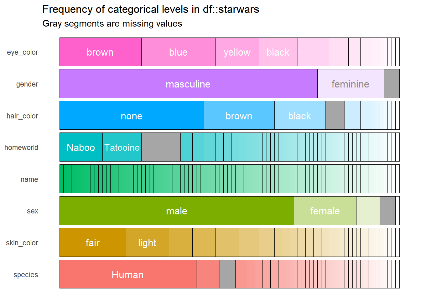
The previous result contains the same information as the df object, but now it is easier, faster, and even easier to interpret. However, this result can be improved, because the variable * name * does not work much in the graph because all the names are different. It can solve by modifying the argument high_cardinality, which means that only those categories that appear a certain number of times say four will be in the plot.
df %>%
    show_plot(high_cardinality = 4)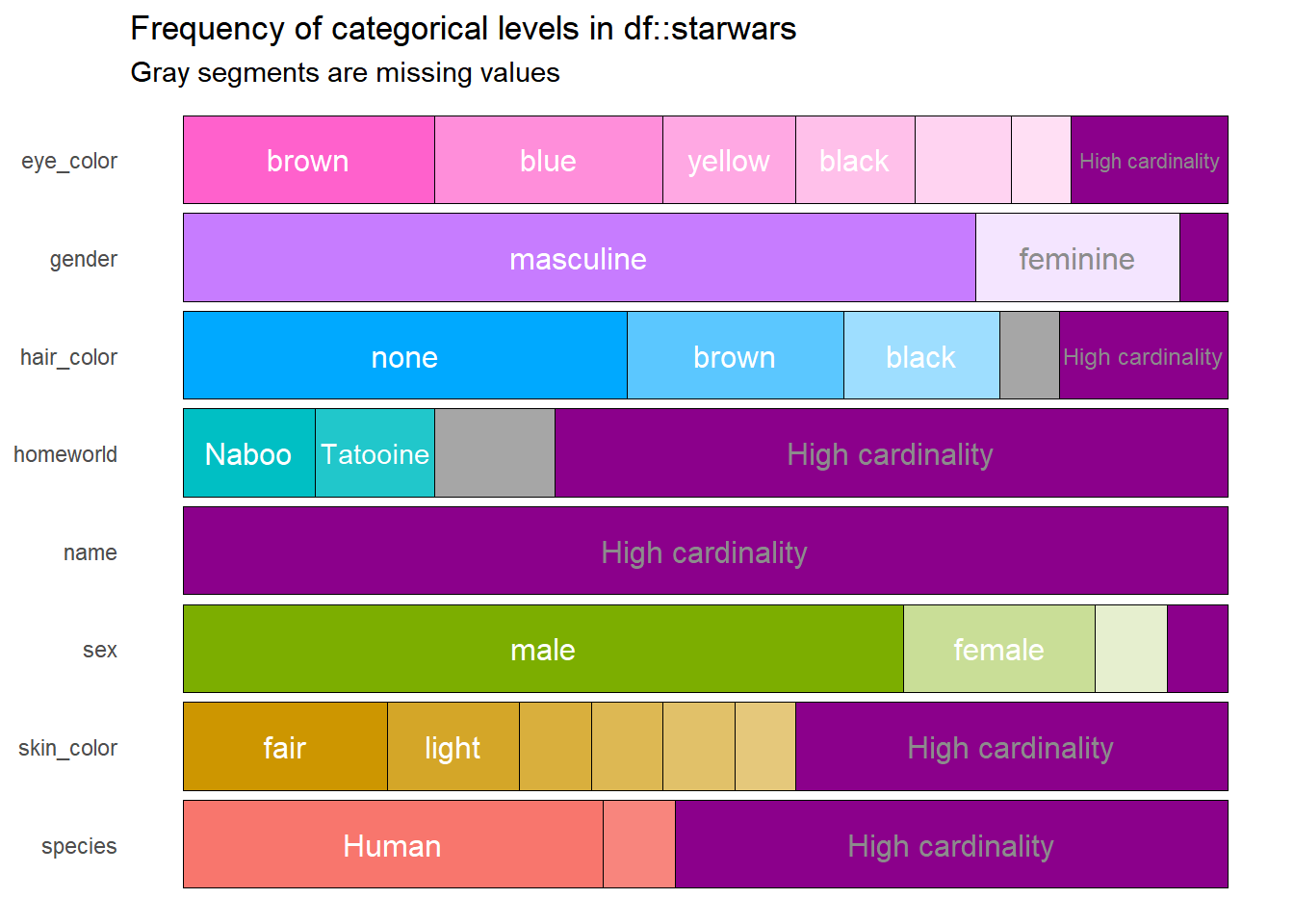
Finally, if the colors are not entirely pleasant, they can be manipulated through the five color palettes offered by the package, we only have to modify the col_palette argument with numbers between one and five to achieve this.
df %>%
    show_plot(high_cardinality = 4, col_palette = 4)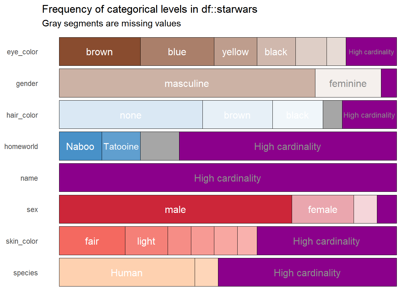
df %>%
    show_plot(high_cardinality = 4, col_palette = 5)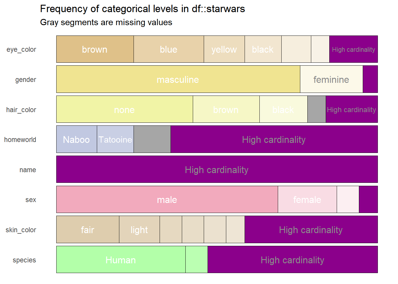
 https://orcid.org/0000-0001-6733-4759